The probability density function (pdf) is a function that completely characterizes the distribution of a continuous random variable.
In this page, we provide concise explanations about the meaning and interpretation of the pdf.
![]()
There are two main ways to specify the probability distribution of a random variable:
assign a probability to each value that the variable can take;
assign probabilities to intervals of values that the variable can take.
Method 1 is used when the set of possible values of the variable is countable (the variable is discrete).
Method 2 is applied if the set is uncountable (the variable is continuous) and Method 1 cannot be used. Method 2 involves the probability density function. Let us see why and how.
Method 1 cannot be employed when the set of possible values is uncountable.
This impossibility is due to a number of fundamental mathematical reasons. For example:
the elements of an uncountable sets cannot be arranged into a sequence; if we attempted to assign probabilities to each possible value of the variable, we would have no order to follow;
even if we managed to assign the probabilities to the single values, we would not be able to check that their sum is equal to 1; in fact, there is no way of summing all the numbers in an uncountable set.
To circumvent this impossibility, mathematicians invented a "trick" that relies on probability density functions and integrals.
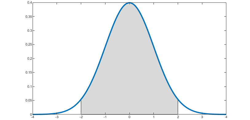
The probability that a continuous random variable takes a value in a given interval is equal to the integral of its probability density function over that interval.
In turn, the integral is equal to the area of the region in the xy-plane bounded by:
the x-axis;
the pdf;
the vertical lines corresponding to the boundaries of the interval.
For example, in the picture below the blue line is the pdf of a normal random variable, and the area of the grey region is equal to the probability that the random variable takes a value in the interval between -2 and 2.
The following is a formal definition.
Definition
The probability density function of a continuous random variable
![]() is a function
is a function
![]() such
that
such
that![[eq2]](/images/probability-density-function__3.png) for
any interval
for
any interval
![]() .
.
The set of values
![]() for which
for which
![]() is called the support of
is called the support of
![]() .
.
Suppose that a random variable
![]() has probability density
function
has probability density
function![[eq5]](/images/probability-density-function__9.png)
In order to compute the probability that
![]() takes a value in the interval
takes a value in the interval
![]() ,
we need to integrate the probability density function over that
interval:
,
we need to integrate the probability density function over that
interval:![[eq6]](/images/probability-density-function__12.png)
It is important to understand a fundamental difference between:
the probability density function, which characterizes the distribution of a continuous random variable;
the probability mass function, which characterizes the distribution of a discrete random variable.
Remember that:
a discrete random variable can take a countable number of values;
a continuous random variable can take an uncountable number of values.
The probability mass function of a discrete variable
![]() is a function
is a function
![]() that gives you, for any real number
that gives you, for any real number
![]() ,
the probability that
,
the probability that
![]() will be equal to
will be equal to
![]() .
.
On the contrary, if
![]() is a continuous variable, its probability density function
is a continuous variable, its probability density function
![]() evaluated at a given point
evaluated at a given point
![]() is not the probability that
is not the probability that
![]() will be equal to
will be equal to
![]() .
As a matter of fact, this probability is equal to zero for any
.
As a matter of fact, this probability is equal to zero for any
![]() because
because![[eq9]](/images/probability-density-function__24.png) where
where
![]() is any primitive (or indefinite integral) of
is any primitive (or indefinite integral) of
![]() .
.
The lecture on zero-probability events provides further explanations about this apparently puzzling result.
Although it is not a probability, the value of the pdf at a given point
![]() can be given a straightforward
interpretation:
can be given a straightforward
interpretation:![]() where
where
![]() is a small increment.
is a small increment.
The proof we are going to give is not
rigorous. Rather, we are focusing on the intuition. For the sake of
simplicity, we assume that the pdf is a continuous function. Strictly
speaking, this is not necessary, although most of the pdfs that are
encountered in practice are continuous (by definition, a pdf must be
integrable; however, while all continuous functions are integrable, not all
integrable functions are continuous). If the pdf is continuous and
![]() is small, then
is small, then
![]() is well approximated by
is well approximated by
![]() for any
for any
![]() belonging to the interval
belonging to the interval
![]() .
It follows that
.
It follows that
![[eq16]](/images/probability-density-function__35.png)
In the above approximate equality, we consider the probability that
![]() will be equal to
will be equal to
![]() or to a value belonging to a small interval near
or to a value belonging to a small interval near
![]() .
In particular, we consider the interval
.
In particular, we consider the interval
![]() .
.
The probability is proportional to the length
![]() of the small interval we are considering.
of the small interval we are considering.
The constant of proportionality
![]() is the probability density function of
is the probability density function of
![]() evaluated at
evaluated at
![]() .
.
Thus, the higher the pdf
![]() is at a given point
is at a given point
![]() ,
the higher is the probability that
,
the higher is the probability that
![]() will take a value near
will take a value near
![]() .
.
Related concepts are those of:
joint probability density function, which characterizes the distribution of a continuous random vector;
marginal probability density function, which characterizes the distribution of a subset of entries of a random vector;
conditional probability density function, which is a pdf obtained by conditioning on the realization of another random variable.
The properties that a pdf needs to satisfy are discussed in the lecture on legitimate probability density functions.
More details about the pdf, examples and solved exercises can be found in the lecture on Random variables.
Previous entry: Prior probability
Next entry: Probability mass function
Please cite as:
Taboga, Marco (2021). "Probability density function", Lectures on probability theory and mathematical statistics. Kindle Direct Publishing. Online appendix. https://www.statlect.com/glossary/probability-density-function.
Most of the learning materials found on this website are now available in a traditional textbook format.