In regression analysis, the variance inflation factor (VIF) is a measure of the degree of multicollinearity of one regressor with the other regressors.
![]()
Table of contents
Multicollinearity arises when a regressor is very similar to a linear combination of other regressors.
Multicollinearity has the effect of markedly increasing the variance of regression coefficient estimates. Therefore, we usually try to avoid it as much as possible.
To detect and measure multicollinearity, we use the so-called variance inflation factors.
Consider the linear
regression![]() where:
where:
![]() is the dependent variable;
is the dependent variable;
![]() are
are
![]() regressors;
regressors;
![]() are
are
![]() regression coefficients;
regression coefficients;
![]() is the error term;
is the error term;
the observations are indexed by
![]() .
.
The linear regression can be written in matrix form
as:![]() where:
where:
![]() and
and
![]() are
are
![]() vectors;
vectors;
![]() is an
is an
![]() matrix;
matrix;
![]() is a
is a
![]() vector.
vector.
If the design matrix
![]() has full rank, then we can
compute the ordinary least squares (OLS) estimator of the vector of regression
coefficients
has full rank, then we can
compute the ordinary least squares (OLS) estimator of the vector of regression
coefficients
![]() as
follows:
as
follows:![]()
Under certain assumptions (see, e.g., the lecture on the
Gauss-Markov
theorem), the covariance matrix of the OLS estimator
is![]()
Therefore, the variance of the OLS estimator of a single coefficient
is![]() where
where
![]() is the
is the
![]() -th
entry on the main diagonal of
-th
entry on the main diagonal of
![]() .
.
If the
![]() -th
regressor has zero mean, we can write the variance of its estimated
coefficient
as
-th
regressor has zero mean, we can write the variance of its estimated
coefficient
as![[eq10]](data:image/gif;base64,R0lGODlhAQABAIAAANvf7wAAACH5BAEAAAAALAAAAAABAAEAAAICRAEAOw==) where
where
![]() is the
R
squared obtained by regressing the
is the
R
squared obtained by regressing the
![]() -th
regressor on all the other regressors.
-th
regressor on all the other regressors.
Without loss of generality, suppose that
![]() (otherwise, change the order of the regressors). We can write the design
matrix
(otherwise, change the order of the regressors). We can write the design
matrix
![]() as a block
matrix:
as a block
matrix:![]() where
where
![]() is the first column of
is the first column of
![]() and the block
and the block
![]() contains all the other columns. Then, we
haveWe
use Schur complements, and in
particular the
formula
contains all the other columns. Then, we
haveWe
use Schur complements, and in
particular the
formula![[eq13]](/images/variance-inflation-factor__36.png) to
write the first entry of the inverse of
to
write the first entry of the inverse of
![]() as:
as:![[eq14]](/images/variance-inflation-factor__38.png) As
proved in the lecture on
partitioned
regressions, the matrix
As
proved in the lecture on
partitioned
regressions, the matrix
![]() is idempotent and symmetric; moreover, when it is post-multiplied by
is idempotent and symmetric; moreover, when it is post-multiplied by
![]() ,
it gives as a result the residuals of a regression of
,
it gives as a result the residuals of a regression of
![]() on
on
![]() .
The vector of these residuals is denoted
by
.
The vector of these residuals is denoted
by![]() Therefore,
Therefore,
![[eq17]](/images/variance-inflation-factor__44.png) If
If
![]() has zero mean, the R squared of the regression of
has zero mean, the R squared of the regression of
![]() on
on
![]() is
Note
that this formula for the R squared is correct only if
is
Note
that this formula for the R squared is correct only if
![]() has zero mean. Then, we can
write
has zero mean. Then, we can
write![]() Therefore,and
Therefore,and
If the
![]() -th
regressor is orthogonal to all the other regressors, we can write the
variance of its estimated coefficient
as
-th
regressor is orthogonal to all the other regressors, we can write the
variance of its estimated coefficient
as![]()
As in the previous proof, we assume without
loss of generality that
![]() .
In that proof, we have demonstrated
that
.
In that proof, we have demonstrated
that![[eq23]](/images/variance-inflation-factor__56.png) If
If
![]() is orthogonal to all the columns in
is orthogonal to all the columns in
![]() ,
then
,
then![]() Therefore,
Therefore,
![[eq25]](/images/variance-inflation-factor__60.png)
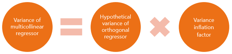
Thus, the variance of
![]() is the product of two terms:
is the product of two terms:
the variance that
![]() would have if the
would have if the
![]() -th
regressor were orthogonal to all the other regressors;
-th
regressor were orthogonal to all the other regressors;
the term
![]() ,
where
,
where
![]() is the R squared in a regression of the
is the R squared in a regression of the
![]() -th
regressor on all the other regressors.
-th
regressor on all the other regressors.
The second term is called the variance inflation factor
because it inflates the variance of
![]() with respect to the base case of orthogonality.
with respect to the base case of orthogonality.
In order to derive the VIF, we have made the important assumption that the
![]() -th
regressor has zero mean.
-th
regressor has zero mean.
If this assumption is not met, then it is incorrect to compute the
VIF as
because
the latter is no longer a factor in the formula that relates the actual
variance of
![]() to its hypothetical variance under the assumption of orthogonality.
to its hypothetical variance under the assumption of orthogonality.
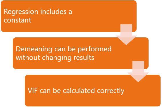
One way to make sure that the zero-mean assumption is met is to run a demeaned regression: before computing the OLS coefficient estimates, we demean all the variables.
As explained in the lecture on partitioned regression, demeaning does not change the coefficient estimates, provided that the regression includes a constant.
Note that a demeaned regression is a special case of a standardized regression. Therefore, we can run a standardized regression before computing variance inflation factors.
We have explained above that the VIF provides a comparison between the actual variance of a coefficient estimator and its hypothetical variance (under the assumption of orthogonality).
By definition, the
![]() -th
regressor is orthogonal to all the other regressors if and only
if
-th
regressor is orthogonal to all the other regressors if and only
if![]() for
all
for
all
![]() .
.
If the
![]() -th
regressor has zero mean, then the orthogonality condition is
equivalent to saying that the
-th
regressor has zero mean, then the orthogonality condition is
equivalent to saying that the
![]() -th
regressor is
uncorrelated
with all the other regressors.
-th
regressor is
uncorrelated
with all the other regressors.
Denote the sample means of
![]() and
and
![]() by
by
![]() and
and
![]() .
We assume that
.
We assume that
![]() .
Then, the sample covariance between
.
Then, the sample covariance between
![]() and
and
![]() is
Therefore,
is
Therefore,
![]() and
and
![]() are uncorrelated.
are uncorrelated.
This is why, if the
![]() -th
regressor has zero mean, the VIF provides a comparison between:
-th
regressor has zero mean, the VIF provides a comparison between:
the actual variance of a coefficient estimator;
the variance that the estimator would have if the corresponding variable were uncorrelated with all the other regressors.
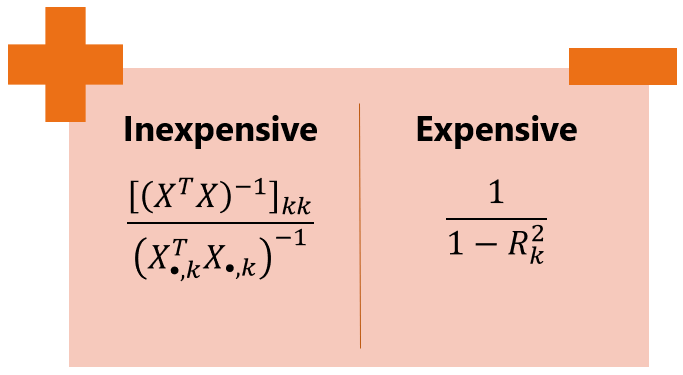
We usually compute the VIF for all the regressors. If there are many
regressors and the sample size is large, computing the VIF
ascan
be quite burdensome because we need to run many large regressions (one for
each
![]() )
in order to compute
)
in order to compute
![]() different R squareds.
different R squareds.
A better alternative is to use the equivalent
formulawhich
can be easily derived from the formulae given above.
We have proved
thatwhich
implies
that
When we use the latter formula, we compute
![]() only once. Then, we use its
only once. Then, we use its
![]() diagonal entries to compute the
diagonal entries to compute the
![]() VIFs.
VIFs.
The numbers
![]() in the denominator are easy to calculate because each of them is the
reciprocal of the inner product of a vector with itself.
in the denominator are easy to calculate because each of them is the
reciprocal of the inner product of a vector with itself.
Here is the final recipe for computing the variance inflation factors:
Make sure that your regression includes a constant (otherwise this recipe cannot be used).
Demean all the variables and drop the constant.
Compute
![]() .
.
For each
![]() compute
compute
![]() .
.
The VIF for the
![]() -th
regressor
is
-th
regressor
is
The VIF is equal to 1 if the regressor is uncorrelated with the other regressors, and greater than 1 in case of non-zero correlation.
The greater the VIF, the higher the degree of multicollinearity.
In the limit, when multicollinearity is perfect (i.e., the regressor is equal to a linear combination of other regressors), the VIF tends to infinity.
There is no precise rule for deciding when a VIF is too high (O'Brien 2007), but values above 10 are often considered a strong hint that trying to reduce the multicollinearity of the regression might be worthwhile.
In the lecture on Multicollinearity, we discuss in more detail the interpretation of the variance inflation factor, and we explain how to deal with multicollinearity.
O'Brien, R. (2007) A Caution Regarding Rules of Thumb for Variance Inflation Factors, Quality & Quantity, 41, 673-690.
Previous entry: Variance formula
Please cite as:
Taboga, Marco (2021). "Variance inflation factor", Lectures on probability theory and mathematical statistics. Kindle Direct Publishing. Online appendix. https://www.statlect.com/glossary/variance-inflation-factor.
Most of the learning materials found on this website are now available in a traditional textbook format.