Autocorrelation is the coefficient of linear correlation between two terms of a sequence of random variables.
Autocorrelation is also called serial correlation.
![]()
The following is formal definition.
Definition
Let
![]() be a sequence of random variables. The autocorrelation coefficient between two
terms of the sequence
be a sequence of random variables. The autocorrelation coefficient between two
terms of the sequence
![]() and
and
![]() is
is![[eq2]](/images/autocorrelation__4.png)
In other words, the autocorrelation coefficient is just the coefficient of linear correlation between two random variables belonging to the same sequence.
Note that the covariance
![]() is called autocovariance.
is called autocovariance.
Remember that a sequence of random variables is said to be covariance stationary (or weakly stationary) if and only if:
all the terms of the sequence have the same
mean:![]()
the covariance between any two terms of the sequence depends only on on how
far apart they are located from each other, and not on where they are located
in the
sequence:![]()
The second of these two properties implies that all the random variables in
the sequence have the same
variance:![]() because
because
![]() .
.
When a sequence is covariance stationary, the autocorrelation coefficient
between two terms of the sequence
![]() and
and
![]() depends only on
depends only on
![]() :
:![[eq8]](data:image/gif;base64,R0lGODlhAQABAIAAANvf7wAAACH5BAEAAAAALAAAAAABAAEAAAICRAEAOw==)
We denote it by
![]() :
and we call it autocorrelation at lag
:
and we call it autocorrelation at lag
![]() (the distance
(the distance
![]() between two terms of the sequence is called lag).
between two terms of the sequence is called lag).
When we observe the first
![]() realizations of a sequence
realizations of a sequence
![]() ,
we can compute the sample autocorrelation at lag
,
we can compute the sample autocorrelation at lag
![]() :
:![[eq11]](/images/autocorrelation__21.png) where
where
![]() is the sample
mean
is the sample
mean
If
![]() is covariance stationary, then the numerator of
is covariance stationary, then the numerator of
![]() is a consistent estimator of
is a consistent estimator of
![]() and the denominator is a consistent estimator of
and the denominator is a consistent estimator of
![]() .
As a consequence,
.
As a consequence,
![]() is a consistent estimator of the autocorrelation at lag
is a consistent estimator of the autocorrelation at lag
![]() .
.
The autocorrelation function (ACF) is the function that maps lags to
autocorrelations, that is,
![]() is considered as a function of
is considered as a function of
![]() (see the examples below).
(see the examples below).
When the mapping is from lags to sample autocorrelations
![]() ,
then we call it sample ACF.
,
then we call it sample ACF.
An ACF plot is a bar chart (or a line chart) that plots the autocorrelation function:
lags are on the x-axis;
the autocorrelations corresponding to the lags are on the y-axis.
Let's look at some examples of ACF and ACF plots.
Suppose that
![]() is a covariance stationary sequence such
that
is a covariance stationary sequence such
that![]() where
where
![]() is a constant and
is a constant and
![]() is an IID sequence of
standard normal
random variables (zero mean and unit variance).
is an IID sequence of
standard normal
random variables (zero mean and unit variance).
Such a sequence is called an autoregressive process of order 1, or AR(1) process (the order is the maximum lag of the sequence on the right hand side of the equation).
Note that
![[eq22]](/images/autocorrelation__37.png) where
we have performed recursive substitutions of
where
we have performed recursive substitutions of
![]() with
with
![]() .
.
By using this expression for
![]() ,
we can easily derive the autocovariance at lag
,
we can easily derive the autocovariance at lag
![]() :
:![[eq24]](/images/autocorrelation__42.png) where:
in steps
where:
in steps
![]() and
and
![]() we have used the
bilinearity of the
covariance operator and in step
we have used the
bilinearity of the
covariance operator and in step
![]() we have used the facts that 1) the covariance of a random variable with itself
is equal to its variance; 2) the covariance between
we have used the facts that 1) the covariance of a random variable with itself
is equal to its variance; 2) the covariance between
![]() and
and
![]() is zero for any
is zero for any
![]() because
because
![]() depends only on
depends only on
![]() for
for
![]() and the sequence
and the sequence
![]() is IID.
is IID.
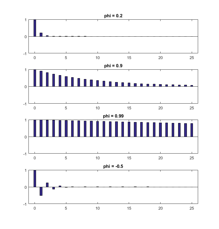
Thus, the autocorrelation at lag
![]() is
is![[eq26]](/images/autocorrelation__54.png)
The following ACF plots show the autocorrelation function for different values
of
![]() .
.
In this example, we show what a sample ACF looks like.
We generate, via Monte Carlo simulations, 200 realizations for each of the four AR(1) processes whose ACFs have been plotted above. The realizations are plotted below.
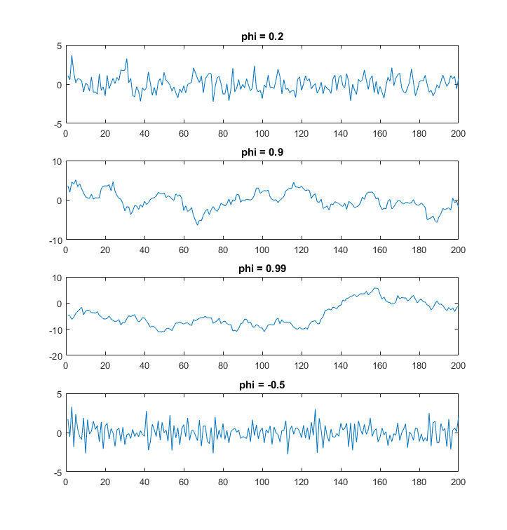
We then compute their sample ACFs, which are plotted below.
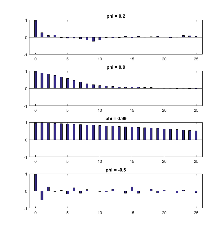
These are the sample versions of the ACFs shown in Example 1. As the sample autocorrelations are noisy estimates of the true autocorrelations, these ACFs do not coincide with those shown in Example 1.
Please cite as:
Taboga, Marco (2021). "Autocorrelation", Lectures on probability theory and mathematical statistics. Kindle Direct Publishing. Online appendix. https://www.statlect.com/fundamentals-of-statistics/autocorrelation.
Most of the learning materials found on this website are now available in a traditional textbook format.